Python with NumPy and pandas

 

This tutorial is adapted from Web Age course  Applied Data Science with Python.

This tutorial aims at helping you refresh your knowledge of Python and show how Python integrates with NumPy and pandas libraries.

Part 1 – Set up the Environment

1. Download and install the latest Google Chrome browser from:

https://www.google.com/intl/en/chrome/browser

2. Install Anaconda on Windows from:

https://www.anaconda.com/distribution/

3. Set Chrome as Your Default Browser

4. Start the command prompt

5. In the command prompt window that opens, create a new working directory c:\Works and then change directory to it using this commands:

mkdir c:\Works
cd c:\Works

 5. Start a new Jupyter working session by running this command:

jupyter notebook

Wait for the Jupyter notebook page to open in the browser.

6. In the New drop-down box in the top right-hand corner of the Jupyter Home page, select Python 3 to create a new notebook.

A new notebook, called Untitled, should initialize.

7. Rename the notebook as Python with NumPy and pandas

Part 2 – Setting up Imports

1. In the currently active input cell, enter the following commands one after another pressing Enter after each line and Shift+Enter to submit the command batch for execution:

import numpy as np
import pandas as pd

The import aliases np and pd are standard for the imported NumPy and pandas libraries, which you should adhere to as well.

Part 3 – Python Refresher

In this part of tutorial, we will review some basics of Python that will help you understand and complete this tutorial. 

So let’s get started …

Python naming convention for variable names is lowercase with words separated by underscores, e.g. this_is_my_variable. The mixedCase is also allowed in contexts where that’s already the prevailing used style.

The None Type

In Python, the closest to null in other languages is None which is a singleton object equal to another None.

1. Enter the following command:

type(None)

You should see the following output:

NoneType

2. Enter the following command:

None == None

You should see the following output:

True

You would usually use the identity operator is to check if the object carries the None value:

n = None
n is None   # True

Version of packages is very important. Here is how you can quickly check a package version.

Printing a Package Version

3. Enter the following command:

np.__version__ 

You should see this output (your version may be higher):

'1.14.0'

The Integer Division

There were some fundamental changes in operations between Python 2 and Python 3.

One of the biggest one is the handling of the integer division.

Python 2 will treat 7/8 as an integer division, returning 0 (performing truncation). Python 3 will convert the factors to float and return a float result (0.875). If you need a-la Python 2 type of integer division, use two slashes //, e.g. 7//8.

String Formatting

Python 2.6+ introduced simple string formatting operator:

s = 'Mr. {1} is {0} years old'.format (45,'Smith')

The s variable will be assigned:

'Mr. Smith is 45 years old'

If you omit indexes (1 and 0) in the placeholders'{}’ like so:

s = 'Mr. {} is {} years old'.format (45,'Smith')

You will have this interpolated string:

'Mr. 45 is Smith years old'

You may need to swap the actual parameters (45,’Smith’) to get what you may really want.

String substringing

For string substringing, Python uses the array notation treating characters in a string as elements in an array.

4. Enter the following commands:

i = '1234567'
i[:3]

You should see the following output:

'123'

Try to guess what output will be for the i[3:] command.

5. Enter the following command to get the last element in the array:

i[-1]

You should see the following output:

'7'

Getting the last element is a frequently used operation in processing Machine Learning data sets as the last element of an array (or the last column in a matrix) is often reserved for the target variable that you want to predict with your model.

And the predictor variables, which come before that last element, can be accessed in an array like so (leaving our the last element):

i[:-1] 

Loops

Here is the common for-loop cycling idiom in Python.

6. Enter the following commands:

for k in range(5):
    print (k)

You should see the following output:

0
1
2
3
4

Note. In Python 3, range() took over from the xrange() function (which was more memory efficient for large ranges) and the latter was dropped.

The range() supports the start (with the default of 0), stop, and step (default is 1) parameters.

Easy Numbers

Python 3.6 introduced the user-friendly large number notation, e.g.

f = 1_222_333.99

which will be interpreted by Python as a floating-point number of 1222333.99.

Note. Python 2 had the int and long types.

Python 3 has only int. Essentially, long was renamed to int. So Python 3 has only one built-in integral type, named int which behaves mostly like the old long type.

The zip Function

The zip() function allows you to iterate over lists passed to it as parameters (you may have two or more lists).

7. Enter the following commands:

x = [1,2,3,4,5]
y = [10,20,30,40,50]
z =['a','b','c','d','e']
[z + '->' + str(x) + ':' + str(y) for x, y, z in zip(x,y,z)]

You should see the following output (of type list):

['a->1:10', 'b->2:20', 'c->3:30', 'd->4:40', 'e->5:50']

List Comprehensions

Comprehensions are constructs that allow sequences to be built from other sequences. Python 2.0 introduced list comprehensions and Python 3.0 extended this functionality to work with dictionaries and sets.

Usually, you use list comprehensions to capture indexes of array elements that satisfy a predicate.

Here is how it works.

8. Enter the following command:

[ i**2 for i in range (1, 5) if (i % 2 == 0)]

You should see the following output (we start with 1, not the default 0):

[4, 16]

It works as follows:

First, the for i in range (1, 5) loop operation kicks in. Then, for each i, the if (i % 2 == 0) predicate is evaluated. If i satisfies the predicate condition (i is even, in our case), i is made available to the power operation (i ** 2).

Basically, the input sequence (range(1, 5)) is translated into the output list [4, 16].

Part 4 – The NumPy Library

At the core of NumPy is its “ndarray” data structure, which is a n-dimensional array.

1. Enter the following commands:

python_list = [1,2,3,4,5]
np_array = np.array([python_list])

np_array is of type numpy.ndarra.

NumPy’s array() function takes a Python list (a rather inefficient bloated data structure) as its input and converts it into a small-footprint nimble data structure using native C-language bridge.

NumPy has a function similar to Python’s range called arange() which acts as a generator of an arithmetic progression sequence.

2. Enter the following command:

np.arange(12) 

You should see the following output:

array([0, 1, 2, 3, 4, 5, 6, 7, 8, 9, 10, 11])

The above array is a simple one-dimensional structure of type numpy.ndarray.

3. Enter the following command:

np.arange(12).shape

The above command will return a tuple that confirms that we have a one-dimensional array:

(12,)

Let’s build a 3×4 matrix (3 rows by 4 columns) from the above one-dimensional array.

4. Enter the following command:

np.arange(12).reshape(3,4)

You should see the following output:

array([[ 0,  1,  2,  3],
       [ 4,  5,  6,  7],
       [8,  9, 10, 11]])

The shape property called on it would show this value (packaged as a tuple):

(3,4)

NumPy supports a wide spectrum of linear algebra operations, like matrix multiplication (through the .dot() method), and the like.

NumPy makes it easy to filter elements in a numpy.ndarray subject to a predicate as well as generate boolean arrays.

5. Enter the following command:

np_array % 2 == 0

You should see the following output (which is a boolean array):

array([[False,  True, False,  True, False,  True]])

6. Enter the following command (which acts as a filter on the target array):

np_array [np_array <= 3]

You should see the following output (the result of a filtering operation):

array([1, 2, 3])

Part 5 – The pandas Library

pandas is an open source, BSD-licensed library that provides high-performance data structures and data analysis tools for the Python programming language. The center piece of pandas is the DataFrame object around which the whole pandas‘ functionality is built.

In this part, we will illustrate the main operations involving the DataFrame object. We will also demonstrate the common idioms related to generating data sets for proof-of-concept Data Science projects.

First, we will create a small 5×2 matrix that we will use as data for a DataFrame object.

Our DataFrame object will have two columns: Sales and Location that represent sales figures per location for some fictitious retail business.

1. Enter the following commands to generate some sales numbers (expressed in, say, million dollars) to be used in the Sales column:

np.random.seed(10)
sales = np.array((100 * np.random.rand (5)).astype(int))
sales

You should see the following output:

array([77,  2, 63, 74, 49])

The np.random.seed(10) command is the common way to seed (set the initial value of) the random generator so that we can reproduce the results at a later time using the same seed value.

Here is how we can generate the Location column values.

2. Enter the following commands:

location = []
for i in range(5):
    location.append('ABCDE'[i]])                
        
location

You should see the following output:

['A', 'B', 'C', 'D', 'E']

Now, let’s combine both arrays into a matrix.

3. Enter the following commands:

data = np.array([sales, location]).T
data

Notice how we transposed (swapped rows for columns) the data matrix using the .T operator.

You should see the following output:

array([['77', 'A'],
       ['2', 'B'],
       ['63', 'C'],
       ['74', 'D'],
       ['49', 'E']], dtype='<U11')

Also notice that the integer values in the first columns have been turned into the String type — you can often observe this behavior when you read data from a file. We will restore the integer type of the first column shortly.

4. Enter the following commands:

df = pd.DataFrame(data, columns = ["Sales", "Location"])
df

Notice how we add the column names to be used in the DataFrame object. Without this configuration, panda’s DataFrame will assume the column names as ordinal values of 0 and 1.

You should see the following output:

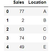In essence, a DataFame object is similar to a relational database table or an Excel spreadsheet.

Now let’s fix the Sales’ column type.

5. Enter the following command:

df.dtypes

You should see the following output:

Sales       object
Location    object
dtype: object

String is disguised as an Object.

Here is the common idiom for changing a DataFrame’s column type to the desired one.

6. Enter the following command:

df.Sales = df.Sales.astype(int)

If you repeat the df.dtypes command now, you should be able to see the following output:

Sales        int32
Location    object
dtype: object  

For numeric types, pandas offers a summary function called describe().

7. Enter the following command:

df.describe()

You should see the following output listing a number of useful descriptive statistics’ metrics like the count of non-None values, the mean, and such like:

	Sales
count	5.000000
mean	53.000000
std	30.553232
min	2.000000
25%	49.000000
50%	63.000000
75%	74.000000
max	77.000000

To get on-line help on a function in Jupyter notebook (functionality delegated to the underlying IPython engine), place a question mark ‘?’ in front of the command (there are some other variations where and when you can place the ? sign).

?df.describe

Here is how you can access values in a DataFrame column (similar to how you can access a column in the SELECT col FROM Table SQL statement).

8. Enter the following command (name auto-completion on DataFrame columns is supported):

df.Location

You should see the values in the Location column.

9. Enter the following command:

df.Sales

The above command is functionally equivalent to the command that uses the loc index accessor, namely:

df.loc[:, 'Sales']

Now, let’s say you want to see the first three values in the Location column of your data frame, here is how you can do this:

10. Enter the following command:

df.loc[:2, 'Location'] 

The index 2 is inclusive (the actual projected indexes are 0, 1, 2).

If you want to see the values in both columns in the rows 1, 2, 3, the command will be:

df.loc[1:3, :]

The last column (:) is kind of a wild card (*) operator applied to all the columns in the DataFrame object.

If you want to take a peek at the last row’s values, use the iloc index accessor.

11. Enter the following command using the iloc index accessor:

df.iloc[-1, :]

You should see the following output:

Sales       49
Location     E
Name: 4, dtype: object

To find the minimum in a numeric column, use this command:

<your_data_frame>.<column_name>.min()

Same command can be used for finding the maximum value; you can also use the describe() method to this end as well.

12. Enter the following command to sort the values in the Sales column in descending order:

df.Sales.sort_values(ascending=False)

You should see the following output:

0    77
3    74
2    63
4    49
1     2
Name: Sales, dtype: int32

Notice how row ids (listed as the first column in the output) have been changed accordingly.

The df.Sales.sort_values() command will sort (the operation does not update data in-place – it is not mutating) the DataFrame object in ascending order.

Now let’s demonstrate how we can add and drop a column in a DataFrame object.

13. Enter the following command to create a new ‘Month‘ column:

df['Month'] = pd.DataFrame(['Jan', 'Feb', 'Mar', 'Apr', 'May'])

14. Enter the following command:

df

The result of the above command will be this DataFrame object;

	Sales	Location	Month
0	77	A	Jan
1	2	B	Feb
2	63	C	Mar
3	74	D	Apr
4	49	E	May

15. Enter the following command to drop the column we just created:

del df['Month']

We are almost done in this tutorial.

Part 6 – Clean-Up

1. Click the Save button in the toolbar.

2. In the menu bar, select File > Close and Halt

The command will shutdown the notebook’s kernel (the sandboxed Python session) and close the interactive edit session.

Keep the browser window open as we are going to use it later.

This is the last step in this tutorial.

Part 7 – Review

In this tutorial, you refreshed your memory (or learned) several things you need to know about Python; you also learned (or refreshed you memory) how to use NumPy and pandas libraries.