Python for Data Science

This tutorial is adapted from Web Age course  Applied Data Science with Python.

This tutorial provides  quick overview of Python modules and high-power features, NumPy library, pandas library, SciPy library, scikit-learn library, Jupyter notebooks and Anaconda distribution.

1.1 Importing Modules

Command 

from lib import x
from lib import x as y

from lib import *

1.2 Listing Methods in a Module

• Use the dir() function:

dir(module_alias), e.g. dir(np)
or
dir('module_name'), e.g. dir('sys')

1.3 Creating Your Own Modules

• Create a Python file, e.g.

# my_utils.py
def foo(a, b):
   return a + b

• Create a directory with the following structure:

├── my_library    	# directory
│ ├── __init__.py   	# empty file, without it, Python will not allow import from a directory
│ ├── my_utils.py		# your module (def …)

• If my_library is in the current working directory of an interpreter, we can import my_utils in the following way:

from my_library import my_utils
my_utils.foo(4, 2)

• When you import a module, its code gets automatically scanned and executed by Python

• To create a runnable application, add the following (highlighted below) code:

def foo(a, b):
   return a + b
if __name__ == "__main__":
# Application entry point is here

1.4 Random Numbers

• Python comes with a pseudo-random (deterministic) number generator

import random   # can alias the import  
random.random()    # a float in a range of [0, 1)
random.randint(x,y)  # an integer in a range of [x,y]

• Note: NumPy offers additional functionality on top of this generator

Notes:

Python uses the Mersenne Twister as the pseudo-random number generator. It produces 53-bit precision floats and has a generation cycle of 2**19937-1 (the cycle is 6002 digits long). The underlying implementation in C, which is both fast and threadsafe.

1.5 Zipping Lists

• The zip() function allows you to iterate over two or more lists passed to it as parameters, for example:

a = [1,2,3,4,5]
b = [10,20,30,40,50]
[str(x) + ':' + str(y) for x, y in zip(a,b)]
Output:
['1:10', '2:20', '3:30', '4:40', '5:50']

1.6 List Comprehension

• Comprehensions are constructs that allow sequences (e.g. lists) to be built from other sequences

  • Python 2 introduced list comprehensions and Python 3 extended this functionality to work with dictionaries and sets

y = 10 
[ i**2 + y for i in range (1, 20) if (i % 2 == 0) ]
Output:
[14, 26, 46, 74, 110, 154, 206, 266, 334]

1.7 Python Data Science-Centric Libraries

• NumPy

• SciPy

• pandas

• scikit-learn

• Matplotlib

1.8 NumPy

• Efficient numerical computing is not Python’s strong point

• NumPy library (http://www.numpy.org/), first released in 2006, addresses Python’s shortcomings in this area

  • The project was a successful attempt to bring together a variety of projects in the space and unify the community around a single array package

  • NumPy is part of SciPy

  • It is open-source software

  • Modeled after Matlab

• At its core, NumPy has an n-dimensional array called “ndarray” that may be shaped as an array or a matrix

• NumPy also offers developers a large collection of functions to work on the ndarray structure

• The ndarray structure replaces Python’s list object

1.9 NumPy Arrays

import numpy as np 
# Aliasing it as np – the accepted convention
# Simple arrays:
a1 = np.array ([1,2,3,4,5])  
# Takes in a Python list as input and outputs a numpy.ndarray object 
a2 = np.arange(5) 
# A numpy.ndarray object holding [0, 1, 2, 3, 4] 
# A matrix structure (note the nested brackets)
m = np.array ([[1,2,3,4], [5,6,7,8]])
m.shape
Output: (2, 4)

1.10 Select NumPy Operations

• Support for vectorization (no-loop ops, uses very fast C code):

10 * np.arange(5) + np.arange(5)
Output:
array([ 0, 11, 22, 33, 44])
np.cos( np.pi * np.array([0,1,2,3]))
Output:
array([ 1., -1.,  1., -1.])

• Filtering:

a = np.array ([1,2,3,4,5])
a [a % 2 == 0]
Output:
array([2, 4])

• Reshaping (in this case, an array into a 4×2 matrix):

m = np.array ([1,2,3,4,5,6,7,8]).reshape(4,2)
Output: a 4x2 matrix

1.11 SciPy

• SciPy (https://scipy.org/) is a Python-based ecosystem of open-source software for mathematics, science, and engineering:

  • statistics

  • linear algebra

  • optimization

  • signal processing (FFT)

  • Note: For the complete list of modules, visit https://docs.scipy.org/doc/numpy-1.6.0/py-modindex.html

• SciPy is built upon the foundational infrastructure of NumPy

Notes:

The SciPy module includes the following sub-packages:

constants: physical constants and conversion factors (since version 0.7.0[5])
cluster: hierarchical clustering, vector quantization, K-means
fftpack: Discrete Fourier Transform algorithms
integrate: numerical integration routines
interpolate: interpolation tools
io: data input and output
lib: Python wrappers to external libraries
linalg: linear algebra routines
misc: miscellaneous utilities (e.g. image reading/writing)
ndimage: various functions for multi-dimensional image processing
optimize: optimization algorithms including linear programming
signal: signal processing tools
sparse: sparse matrix and related algorithms
spatial: KD-trees, nearest neighbors, distance functions
special: special functions
stats: statistical functions
weave: tool for writing C/C++ code as Python multiline strings

1.12 pandas

• pandas (https://pandas.pydata.org/) is an open source library that provides high-performance, memory-efficient, easy-to-use data structures, as well as support for data manipulation and analysis for Python

• The core pandas’ data structure is the DataFrame object with integrated indexing similar to a relational table, Excel spreadsheet, and similar tabular data set containers

  • The major influence was R’s DataFrame object

• Through dataframes, pandas offers compact and efficient interfaces for reading and writing data between its data structures and files stored in different formats: CSV, Microsoft Excel, SQL databases, and the fast HDF5 format

• Dataframes offer integrated handling of missing data points and other mechanisms for patching data sets

• Supported operations include: data set reshaping, grouping, aggregation, pivoting, joining, querying, and similar operations

1.13 Creating a pandas DataFrame

import pandas as pd
import numpy as np
# You build a DataFrame as a matrix (array of arrays)
m = np.array ([1,2,3,4,5,6,7,8]).reshape(4,2)
df = pd.DataFrame(m, columns = ["Col1", "Col2"])
# Now you have this structure:
	Col1	Col2
0	1	2
1	3	4
2	5	6
3	7	8

1.14 Fetching and Sorting Data

df.Col1 # or df['Col1']
# Col1 values with the their indexes as the left-most column
Output:
0    1
1    3
2    5
3    7
Name: Col1, dtype: int32
df.iloc[1, :] 
# Getting the second row via its index
Output:
Col1    3
Col2    4
Name: 1, dtype: int32 
df.Col2.sort_values(ascending=False)
# Sorting values in descending order (ascending order is default)
Output:
3    8
2    6
1    4
0    2
Name: Col2, dtype: int32

1.15 Scikit-learn

• scikit-learn (http://scikit-learn.org/) is a Python module for machine learning built on top of SciPy

• Supports algorithms in these areas:

  • Classification

  • Clustering

  • Data preprocessing (feature extraction and transformation)

  • Dimensionality reduction (deals with data multicollinearity and variance reduction)

  • Model selection (comparing, validating, and improving model accuracy)

  • Regression

1.16 Matplotlib

• Matplotlib (https://matplotlib.org/) is a Python library for graphing and visualization

• Depends on NumPy

• With Matplotlib you can generate plots, histograms, bar charts,scatter plots, etc., with just a few lines of code

• Matplotlib’s main focus is 2D plotting; 3D plotting is possible with the mplot3d package

1.17 Python Dev Tools and REPLs

• In addition to the standard Python REPL, Python development is supported through these developer systems:

  • IPython

  • Jupyter with Python kernel (runtime)

  • Visual Studio Code’s Python plug-in

1.18 IPython

• IPython (Interactive Python) is a command shell that, in addition to Python, supports other computing languages as well

• Originally released in 2001

• Offers code introspection with name auto-completion (on Tab) and command history

• Supports in-line plotting

• In addition to the primary single-user development on a user machine, it can also manage parallel computing clusters using asynchronous status callbacks and/or MPI

• In 2014, the original author, Fernando Pérez, announced a spin-off project from IPython called Project Jupyter with IPython acting as Jupyter’s processing engine

1.19 Jupyter

• Jupyter is a browser-based Python REPL serviced by an embedded web server

  • This Jupyter architecture allows for a remote access (that can be secured)

• Depends on IPython and allows you to use multiple versions of Python (providing their runtimes are installed)

• Supports other languages as well:

  • Julia, R, Haskell, and Ruby

• Central to Jupyter development model is notebook that allows you enter, execute, and mark up code (for documentation and/or simple comments)

  • Notebook files are physical files with extension .ipynb automatically saved in your working directory served by the web server

  • You can have multiple Python notebook sessions running concurrently, each receiving its own Python interpreter sandbox

• You start Jupyter by running this command:

jupyter notebook

Notes:

The name Jupyter is an indirect acronym of the three core languages it was designed for: JUlia, PYThon, and R.

1.20 Jupyter Operation Modes

• Developers use a Jupyter notebook in two modes:

  • Command mode (CM)

    • Visually indicated by a blue left-hand border line of the current cell

  • Edit mode (EM)

    • Visually indicated by a green left-hand border line of the current cell

• When you start a notebook, it opens in EM, ready to accept your commands

• To switch to CM, press Esc

• To switch back to EM, click your mouse in a cell or press Enter

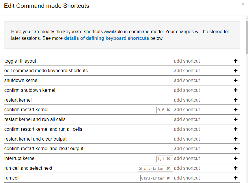
1.21 Jupyter Common Commands

• Basic edit mode (EM) commands:

  • Shift+Enter – run code in the current cell and add a new cell below for the next command

  • Ctrl+Enter – run code in the current cell and switch to CM; if you have multiple selected cells (you can do it in CM), code in all the selected cells is executed

• Basic CM commands:

  • a – add a cell above the current cell

  • b – add a cell below the current cell

  • c – copy a cell (Ctrl-v to paste it)

  • d – delete the current cell

• If you need to re-execute commands in your notebook (All, All Above, or All Below) use the Cell menu option in the menu bar

• Review Jupyter’s help (the Help menu option) to learn about available command shortcuts

Notes:

You can preview and edit the command shortcuts by navigating to Help > Edit Keyboard Shortcuts using the menu bar. Unfortunately, for now, Jupyter does not support macros / scripting.

1.22 Anaconda

• Anaconda is a distribution of Python along with its frequently used packages (NumPy, SciPy, pandas, scikit-learn, etc.)

• Comes with its package manager called conda that helps you list, update and otherwise manage packages

• Anaconda also includes Jupyter

Notes:

The conda package manager supports the following commands:

Create a new conda environment from a list of specified packages

1.23 Summary

• In this tutorial, we discussed the following topics:

  • Python module import considerations, zip and list comprehension commands

  • NumPy

  • pandas

  • SciPy

  • IPython

  • Jupyter notebooks

  • Anaconda Python distribution