This tutorial is adapted from Web Age course Practical Machine Learning with Apache Spark.
6.1 Python Dev Tools and REPLs
In addition to the standard Python REPL, Python development is supported through these tools and systems: IPython, Jupyter with Python kernel (runtime), Visual Studio Code’s Python plug-in, PySpark (integrated with Python REPL).
6.2 IPython
IPython (Interactive Python) is a command shell that, in addition to Python, supports other computing languages as well. It was originally released in 2001. It offers code introspection with name auto-completion (on Tab) and command history. It supports in-line plotting. In addition to the primary single-user development on a user machine, it can also manage parallel computing clusters using asynchronous status callbacks and/or MPI. In 2014, the original author, Fernando Pérez, announced a spin-off project from IPython called Project Jupyter with IPython acting as Jupyter’s processing engine.
6.3 Jupyter
Jupyter is a browser-based Python REPL serviced by an embedded web server. This Jupyter architecture allows for a remote access (that can be secured). Depends on IPython and allows you to use multiple versions of Python. (providing their runtimes are installed). It supports other languages as well like Julia, R, Haskell, and Ruby. Central to Jupyter development model is a notebook that allows you enter, execute, and mark up code (for documentation and/or simple comments). Notebook files are physical files with extension .ipynb automatically saved in your working directory served by the web server. You can have multiple Python notebook sessions running concurrently, each receiving its own Python interpreter sandbox .
You start Jupyter by running this command:
jupyter notebook
6.4 Jupyter Operation Modes
Developers use a Jupyter notebook in two modes:
Command mode (CM) – Visually indicated by a blue left-hand border line of the current cell.
Edit mode (EM)– Visually indicated by a green left-hand border line of the current cell.
When you start a notebook, it opens in EM, ready to accept your commands. To switch to CM, press Esc and to switch back to EM, click your mouse in a cell or press Enter.
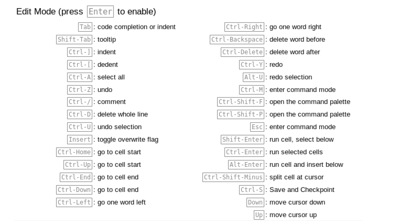
6.5 Basic Edit Mode Shortcuts
Shift+Enter – run code in the current cell and add a new cell below for the next command
Ctrl+Enter – run code in the current cell and switch to CM; if you have multiple selected cells (you can do it in CM), code in all the selected cells is executed.
Shift+Tab – in-context help (tooltip)
Ctrl-Shift-Minus – split cell at cursor
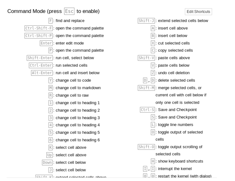
6.6 Basic Command Mode Shortcuts
a – add a cell above the current cell
b – add a cell below the current cell
c – copy a cell (Ctrl-V to paste it)
d – delete the current cell
M – change the cell type from code (default) to markdown
Y – change the cell type to code
1 – change cell to heading 1 (2 for heading 2, etc.)
Note: If you need to re-execute commands in your notebook (All, All Above, or All Below) use the Cell menu option in the menu bar
Review Jupyter’s help (the Help menu option) to learn about available command shortcuts.
 6.7 Summary

In this tutorial, we learned Python-based REPLs and Jupyter notebooks.