This tutorial is adapted from Web Age course Practical Machine Learning with Apache Spark.
8.1 Types of Machine Learning
There are three main types of machine learning (ML), unsupervised learning, supervised learning, and reinforcement learning. We will be learning only about the unsupervised and supervised learning types.
8.2 Supervised vs Unsupervised Machine Learning
In essence, unsupervised learning (UL) attempts to extract patterns without much human intervention; supervised learning (SL) tries to fit rules and equations. SL defines a target variable that needs to be predicted / estimated by applying an SL algorithm using predictor (independent) variables (features). Classification and regression are examples of SL algorithms. SL uses labeled examples. SL algorithms are built on top of mathematical formulas with predictive capacity. UL is the opposite of SL. UL does not have a concept of a target value that needs to be found or estimated. Rather, a UL algorithm, for example, can deal with the task of grouping (forming a cluster of) similar items together based on some automatically defined or discovered criteria of data elements’ affinity (automatic classification technique). UL uses unlabeled examples.
Notes:
Some classification systems are referred to as expert systems that are created in order to let computers take much of the technical drudgery out of data processing leaving humans with the authority, in most cases, to make the final decision.
8.3 Supervised Machine Learning Algorithms
Some of the most popular supervised ML algorithms are Decision Trees, Random Forest, k-Nearest Neighbors (kNN), Naive Bayes, Regression (linear simple, multiple, locally weighted, etc.) and Support Vector Machines (SVMs).
8.4 Classification (Supervised ML) Examples
Identification of prospective borrowers who are likely to default on their loans (based on historical observations), Spam detection and Image recognition (a smiling face, a type of a musical instrument).
8.5 Unsupervised Machine Learning Algorithms
Some of the most popular unsupervised ML algorithms are k-Means, Hierarchical clustering, Gaussian mixture models. Dimensionality reduction falls into the realm of unsupervised learning: PCA, Isomap.
8.6 Clustering (Unsupervised ML) Examples
Some of the examples are Building groups of genes with related expression patterns, Customer segmentation, Grouping experiment outcomes and Differentiating social network communities.
8.7 Choosing the Right Algorithm
The rules below may help you get your direction but those are not written in stone:
- If you are trying to find the probability of an event or predict a value based on existing historical observations, look at the supervised learning (SL) algorithms. Otherwise refer to the unsupervised learning(UL).
- If you are dealing with discrete (nominal) values like TRUE:FALSE, bad:good:excellent, etc., you need to go with classification algorithms of
SL. - If you are dealing with continuous numerical values, you need to go with regression algorithms of SL.
- If you want to let the machine categorize data into a number of groups, you need to go with clustering algorithms of UL.
8.8 Terminology: Observations, Features, and Targets
In data science, machine learning (ML), and statistics, features are variables that are used in making predictions; they are also called predictors or independent variables. They are the inputs of your model. A feature is similar to a relational table’s column (entity attribute, or property). The value that you predict using features is referred to as a target, or response, or outcome, or predicted variable, or dependent variable. This is the output of your model. An observation is the registered value of a particular variable (feature) like temperature, an individual product’s price, etc. An observation is like a table’s row or record. In ML, observations are often referred to as examples.
8.9 Representing Observations
Vector notation is widely used to represent observations. The observation vector’s elements are features that are usually denoted as x1, x2, x3, … xN. Generally, those elements may be vectors themselves, so X below may, in fact, reference a matrix – an array (vector) of arrays:
X {x1, x2, x3, … xN}
8.10 Terminology: Labels
A label is a type of object or a value that we assign to an observation or what we are trying to predict. You can have labeled and unlabeled observations (examples); the former are mostly used in classification, the latter are found in clustering (unsupervised learning). In classification, labeled examples are used to train the model; after that the trained model is fed unlabeled observations (examples) to have the model infer (intelligently guess) the labels of the observations.
Label examples:
- Software defect severity levels: Blocker, Critical, Major, Minor
- Trading recommendations: Buy, Sell, Hold
- E-mail categories: Spam, Non-spam
8.11 Terminology: Continuous and Categorical Features
Features can be of two types: continuous, or categorical. Categorical features, in turn, are divided into nominal and ordinal.
8.12 Continuous Features
Continuous features represent something that can be physically or theoretically measured in numeric values, e.g. blood pressure, size of a black hole, plane speed, humidity etc. Regression models work with continuous features for learning and predicting and help answer this type of questions,” Given our past sales, what is the expected sales figure for the next month?”
8.13 Categorical Features
Categorical variables are discrete, enumerated types that can be ordinal or nominal, like hurricane category, gender, security threat level, city regions, car types, etc. The nominal and ordinal categories can be illustrated using playing cards. Nominal categories are represented by suits: hearts, diamonds, spades, and clubs (generally, there is no ordering in suites and if one exists, it is game-specific). Ordinal categories are (with some variations) represented by the ranks in each suite (Ace, 2, 3, 4, …., J, Q, K).
8.14 Common Distance Metrics
A data point is a value at the intersection of a feature (column) and an instance of the observation instance (row). Data science (including ML) uses the concept of a distance between data points as a measure of object similarity. For continuous numeric variables, the Minkowski distance is used, which has this generic form:
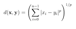
The Minkowski distance has three special cases:
- For p=1, the distance is known as the Manhattan distance (a.k.a the L1 norm)
- For p=2, the distance is known as the Euclidean distance (a.k.a. the L2 norm)
- When p → +infinity, the distance is known as the Chebyshev distance
In text classification scenarios, the most commonly used distance metric is Hamming distance.
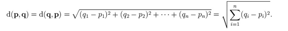
8.15 The Euclidean Distance
The most commonly used distance in ML for continuous numeric variables is the Euclidean distance . In Cartesian coordinates, if we have two points in Euclidean n-space: p and q, the distance from p to q (or from q to p) is given by the Pythagorean formula:

8.16 What is a Model
A model is a formula, or an algorithm, or a prediction function that establishes a relationship between features (predictors) and labels (the output / predicted variable). A model is trained to predict (make inference of) the labels or predict values. There are two major life-cycle phases of a model:
Model training (fitting) – You train or let your model learn on labeled observations (examples) fed to the model
Inference (predicting)- Here you use your trained model to calculate / predict the labels of unlabeled observations (examples) or numeric values
8.17 Model Evaluation
Once you have your ML model built, you can (and should) evaluate the quality of your model, or its predictive capability (i.e. how well it can do predictions). Your model should have the ability to make accurate predictions (or generalize) on new data (not seen during training). The model evaluation is specific to the estimator you use and you need to refer to the estimator’s documentation page. In this module, we will demonstrate how to evaluate various models.
8.18 The Classification Error Rate
A common measure of a classification model’s accuracy is the error rate which is the number of wrong predictions (e.g. classification of test observations) divided by the total number of tests. In the ideal world (when you have a perfect training set and your test objects have strong affinity with some classes), your model makes predictions with no errors (the error rate is 0). On the other side of the spectrum, an error rate of 1.0 indicates a major problem with the training set and/or ambiguous test objects. Error tolerance levels depend on the type of the model.
8.19 Data Split for Training and Test Data Sets
In ML, the common practice is not to use the same data used for training your model and testing it. If you must use the same data set for training and testing your ML model (e.g. due to limited availability of the source data), you need to split the data into two parts so that you have one data set for training your model, and one for testing. In this case, your trained model is validated on data it has not previously seen, which gives you an estimate of how well your model can generalize (fit) to new data. There are many variations of the splitting techniques, but the most common (and simple) one is to allocate about 70-80% of the initial data for training and 20-30% for testing.
8.20 Data Splitting in PySpark
There are a number of considerations when performing a data split operation. Observations (records) must be selected randomly to prevent record sequence bias. Every labeled record (for classification models) should have a fair share in both training and testing data sets. PySpark simplifies this operation through the randomSplit() method of the DataFrame object:
train_df, test_df = input_df.randomSplit()
8.21 Hold-Out Data
Observations that are set aside for testing and not used during training are called “holdout” data. Holdout data is used to evaluate your model’s predictive capability and its ability to generalize to data other than the data the model saw during the trained step.
8.22 Cross-Validation Technique
A popular model validation technique used in cases when it is not practical to split the source dataset into training and test parts (e.g. due to the small
data set’s size). The most commonly used variation of this technique is called k-fold crossvalidation, which is an iterative process that works as follows:
- First you divide the source dataset into k equal folds (parts)
- Each of the folds takes turns to become the hold-out validation set (test data), the rest k-1 folds are merged to create the training data set
- Process repeats for all k folds
- When done, calculate the average accuracy across all the k folds
8.23 Spark ML Overview
Spark ML offers the following modalities:
ML Algorithms: common learning algorithms such as classification, regression, clustering, and collaborative filtering
Featurization: feature extraction, transformation, dimensionality reduction, and selection
Pipelines: tools for constructing, evaluating, and tuning ML Pipelines
Persistence: saving and load algorithms, models, and Pipelines
Utilities: linear algebra, statistics, data handling, etc.
8.24 DataFrame-based API is the Primary Spark ML API
As of Spark 2.0, the RDD-based APIs in the spark.mllib package have entered maintenance mode. RDD-based API in spark.mllib will be still supported with bug fixes. No new features will be added to the RDD-based API. The RDD-based API is expected to be removed in Spark 3.0. The primary ML API for Spark is now the DataFrame-based API in the spark.ml package. DataFrames provide a uniform and more developer-friendly API than RDDs. DataFrames support feature transformations and building ML pipelines.
8.25 Estimators, Models, and Predictors
ML systems use the terms model, estimator and predictor in most cases interchangeably.
8.26 Descriptive Statistics
Descriptive statistics helps quantitatively describe data sets. This discipline provides numerical measures to quantify data. The typical measures of continuous variables are: mean, median and mode (central tendency measures); the minimum and maximum values of the variables, standard deviation; (or variance), kurtosis and skewness (measures of variability ). Essentially, here you find the central tendency and spread of each
continuous feature (variable). To describe categorical variables, you can use frequency, or percentage table to find the distribution of each category
8.27 Data Visualization and EDA
Descriptive statistics is supplemented by such visualization modalities and graphical forms as Histograms, Heat Maps, Charts, Box Plots, etc.
Data visualization is an activity in exploratory data analysis (EDA) aimed at discovering the underlying trends and patterns, as well as communicating the results of the analysis. Business intelligence software vendors usually bundle data visualization tools with their products.
8.29 Correlations
Correlation describes the relationship or association between two variables. Correlation coefficients are used to measure the degree to which two
variables are associated. The sign (+ or -) of the correlation coefficient indicates the direction of the relationship with the ‘+’ sign indicating the positive relationship and ‘–’ the inverse one. The value of the coefficient indicates the strength of the relationship. Correlation coefficients range from 0 indicating that there is no observable relationship up to 1 for absolutely strong relationship.